KLM Remote Sensing/ Google Earth

This KLM data from the VEGETATION program. It is remote sensing of "terrestrial vegetation cover...at the global level." The data is obtained through the VEGETATION1 and VEGETATION2 sensors aboard the SPOT4 and SPOT5 satellites. More information can be found at www.spot-vegitation.com. In using the KLM with Google Earth, One is able to review data from any point on the globe, as well as move through time samples to compare data over time.

Hypsometric Map

This map uses a hypsometric color display to show elevation. In this case the darker green areas are closer to sea level with the progressively brown to tan to white areas marking higher to higher elevations. This map shows only the contiguous United states. In reality the slope continues under sea level to deep sea trenches. Maps that do show underwater topography usually use light blue to denote sea level with progressively darker shades of blue showing increasing depth.

The above image can be found at www.theodora.com/maps/new9/usa_elevation_map.gif

Public Land Survey System (PLSS) Map

The above shows the state of Alabama divided by the meridians and lines of the PLSS. Highlighted in blue is Franklin County. A larger scale look at Franklin County with PLSS divisions is below.

The above map shows Franklin County as a whole, divided by the PLSS system. We will look closer, below, at T6S, R15W. This means we are looking at portion of land 6 Townships south of the Base Line, and we are located in a land portion 15 sections west of Principal Meridian R.


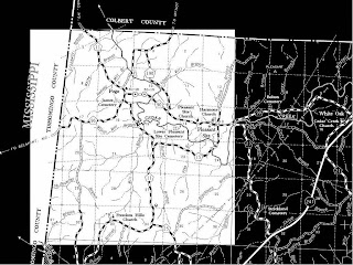
As seen above, state and local borders do not necessarily align with the PLSS System. In particular the difference between the state border on the north from the PLSS system is reflective of the difference between the projections and the PLSS overlay.

All of the above maps can be found at http://www.rootsweb.ancestry.com/~alfrankl/landrecords.htm

Cadastral Map

The above map is a cadastral map for Logan City, Australia. This small-scale map (relative to the one below) obscures some fo the fine detail of a larger scale, but it does allow one to see the changes in relative size of properties in different areas of the city. It would seems there are areas of relatively high population density (or property density, anyway) in the right and top of the map.

On this larger scale map of the same region one can see finer detail, including measurements and boundaries for the individual properties, as well as owner names. It would seem that some sort of meets and bounds measuring system was utilized. I make this inference based on the use of the river on the right as a boundery. This would likey change over time (especially considering the meandering profile of the river).

The original can be found at http://www.logan.qld.gov.au/LCC/logan/history/publications/RidgetoRidgeRecollectionsfromWoodridgetoParkRidge.htm

Thematic Map

http://www.stats.indiana.edu/maptools/maps/thematic/indiana/luxurycars03.gif

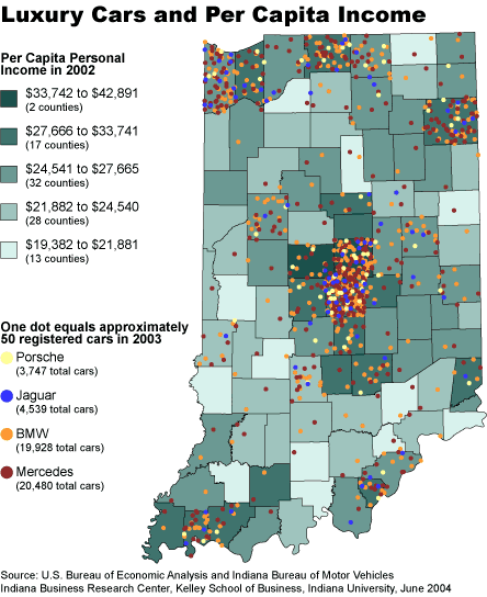
I particularly like this thematic map because it follows two data streams and manages to depict them each clearly. This particular map chooses to use a Choropleth Map to represent the average distribution of income. This base is overlapped with a Dot Distribution map with multiple colors to represent various high-end cars. This combination of grey-tone (well, greenish-blue tone) and colored dotes allows the observer to see the correlation between income and luxury car sales with relative ease. Overall I found this to be a decent representation of the thematic map.

Topographic Map

www.lib.utexas.edu/topo/texas/txu-oclc-50141851-austin_west-1988.jpg


The above map is a depiction of western Austin including elevation changes. In this representation each line represents a 20 foot change in elevation. Also included are roadways, municipalities and local points of interest. In comparing this to the planimetric map you can see the amount of information missing in the planimetric version.

Planimetric Map

www.lib.utexas.edu/maps/texas/austin_1985.jpg

The above map features the city of Austin. The information contained the the map includes natural features such as rivers and wooded areas, but the main focus is on man-made features. Of most importance are roadways and distinguishing between rural and suburban regions. Also present are the names and locations of individual municipalities, roads, and rivers, as well as points of interest such as airports, theme parks and camp grounds. Notably missing is any elevation information. The surface is viewed as if there are no changes in elevation from one area to another. (i.e. plane = planimetric) Compare to Topographic map of the same region.